Creating a Dynamic Lab Environment with vEOS and GNS3 - Part I

GETTING STARTED

Preliminary Installation Setup

Install GNS3

Install VirtualBox

Get ahold of the .vmdk and aboot.iso files

It is recommended to install VirtualBox AFTER you install GNS3 to avoid problems with GNS3 detecting VirtualBox.

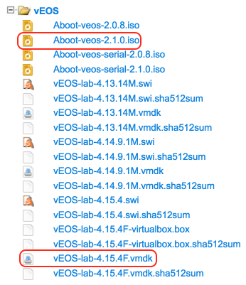
Go to www.arista.com, and go to Support > Software Download.  The two files you’ll want are the .vmdk file as well as the Aboot .iso file:

Creating the Management Network

To simulate an out-of-band management network, we will create a vboxnet interface, similar to a loopback interface, on our laptop.  This will also allow us to interact with our virtual machines via SSH, etc.

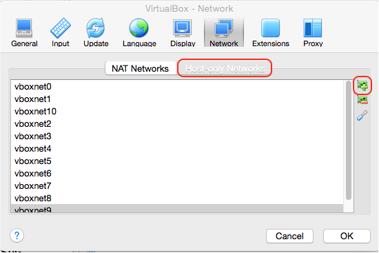
Open VirtualBox, go to Preferences, and click Network. Select “Host-only Networks”, and then click the NIC adapter image with a plus symbol on it to add a new host-only network if there isn’t one already:

Select your newly-created vboxnet and click the screwdriver icon to configure it:

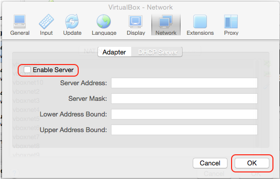
We’re going to be using ZTP to provision our switches, so select “DHCP Server”, ensure “Enable Server” is unchecked, and then click OK:

Verify you have a new interface reflecting your vboxnet configuration:

SETTING UP vEOS

Creating a Base Image

You’ll want a nice, clean base image to create clones from.  

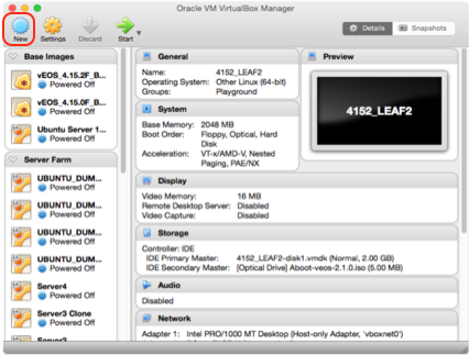
To begin, in VirtualBox, click New:

Give your base image a name.  Use the drop-down menus to set the Type to “Linux”, the Version to “Other Linux (64-bit)”, and then click Continue:

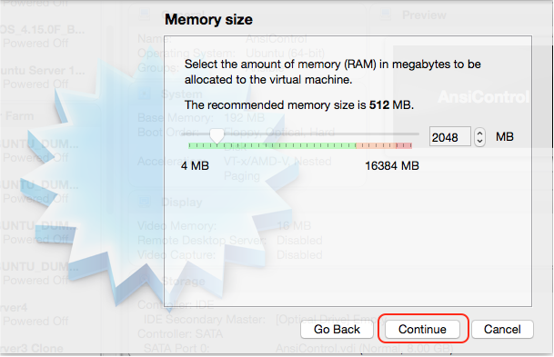
Set the memory allocation to 2048, and then click Continue:

Select “Use an existing virtual hard disk file”, select the .vmdk file you downloaded earlier, and click Create:

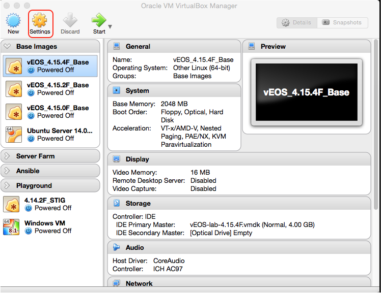
Our base image has been created, but now must be configured.  Select the new base image, and click Settings:

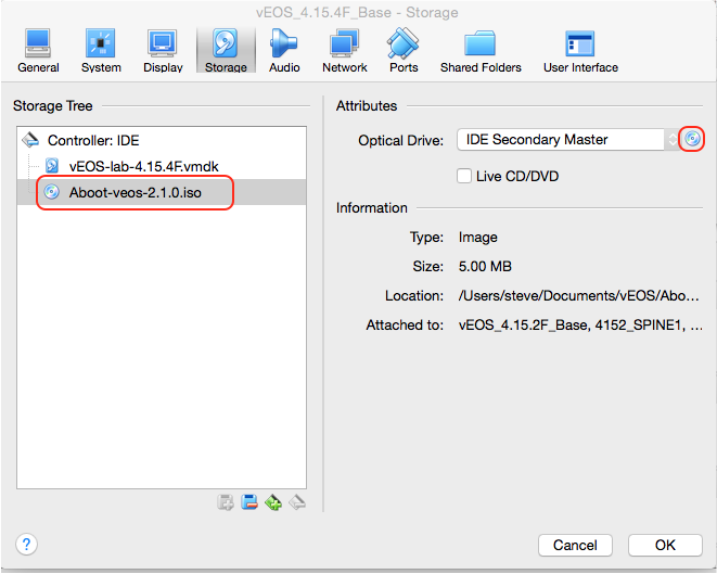
Click Storage, and then use the drop-down menu to set the second entry under “Controller: IDE” to IDE Secondary Master, then click the small CD icon and select the Aboot.iso file downloaded earlier

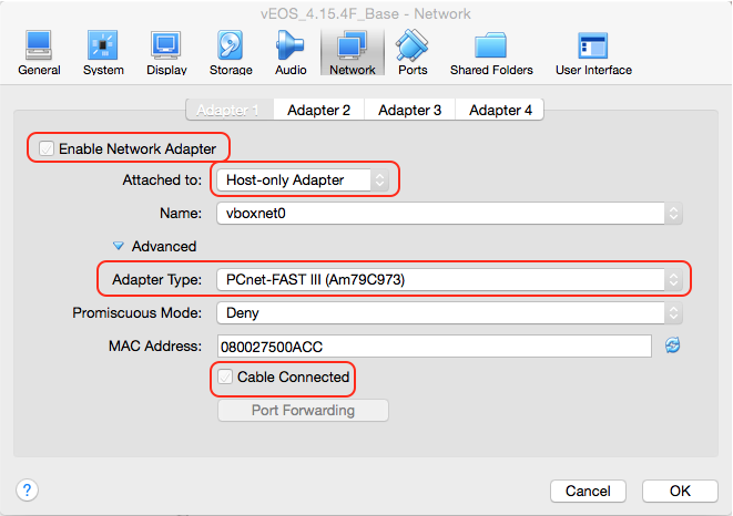
Click Network, select Adapter 1, ensure “Enable Network Adapter” is checked, and use the drop-down menu to select “Host-only Adapter”.  Ensure the Name is populated with the management network created in the previous section, use the drop-down menu to set the Adapter Type is set to “PCnet-FAST III”, and ensure that “Cable Connected” is checked. Click OK to save your changes:

Leave the rest of the Adapters alone - these will be configured for you by GNS3 later.

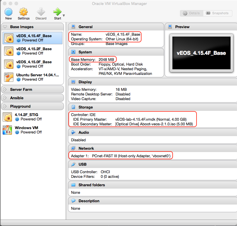
Verify your base image settings and launch the VM to verify it successfully boots:

TIP! At this point, you have a decision to make.  You can either leave the base image as-is and configure everything on the clones that you will make, or if there’s something that will be configured on every clone, such as a username, you could configure this in your base image so that you won’t have to do it on your clones.  For our lab though, we’re going to be provisioning everything with ZTP and Ansible, so I’m going to leave the base image as raw as possible. If you noticed, we created a host-only adapter in our base image so that every time we create a clone, it will already have its first adapter be its management connection.  You’ll see why later.

Creating Clones

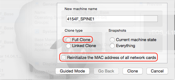
If you haven’t already, shut down your base image.  Now, in VirtualBox, right-click it and select “Clone”.  Click “Expert Mode” - because you’re clearly too awesome for that guided nonsense (And doing it this way is just quicker).  Give your clone a name, ensure that “Full Clone” and “Reinitialize the MAC address of all network cards” is selected, and then click Clone - repeat as necessary to create additional clones:

WARNING! This part is very important.  If you select “Linked Clone”, your clone will be linked to the base image instead of creating its own file.  This means if you accidentally choose to delete all files when you delete your clone later, it will also effectively delete your base image as well.   If you do not select “Reinitialize the MAC address of all network cards”, all clones will have the same MAC address as your base image, and you can imagine the fun that will create in your virtual network.

GETTING STARTED IN GNS3

Adding VMs to GNS3

GNS3 has very tight integration with VirtualBox.  As you create connections between your vEOS instances, server VMs, etc., GNS3 takes care of all configuration needed on your VirtualBox VMs for you - no manual configuration needed inside of VirtualBox itself for each new connection.  

To get started, we’ll need to add our newly-minted cloned vEOS instances to GNS3.  Open GNS3, start a new project, and then open Preferences.  Go to VirtualBox > VirtualBox VMs, click New, use the drop-down menu to select your newly-created clones, and then click Finish - repeat as necessary:

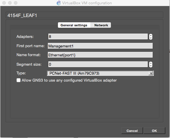
Select your VM and click Edit. Under “Network”, configure the following and then click Ok, repeating as necessary for each VM:

NOTE At the time of this writing, VirtualBox can support a maximum of 8 adapters.  Refer to the article in “Resources/Recommended Reading” for details.  The first adapter will be your management interface, hence the “First port name:”, and then you’ll have an additional 7 interfaces to play with.

TIP! If you want your VM to cosmetically appear more like a switch in GNS3, under “General Settings”, set the Category to “Switches”, and change the Symbol to “Multilayer Switch”.

Click Apply, and then click OK to exit.

Now that our vEOS VMs are configured in GNS3, we can start building our virtual network. On the main project screen, click “Browse All Devices”, and then drag-and-drop your VMs onto the topology panel (the center panel):

Click “Add a Link”, click one VM, select “Ethernet1”, and connect it to your other VM on the same interface:

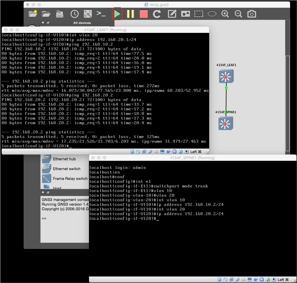
Click “Start/Resume all devices”, and when the VMs are finished booting, setup some VLANs and SVIs and verify you have connectivity:

Great!  Let’s move on to providing “bare-metal” provisioning with ZTP.

How Rapid Spanning Tree Protocol (RSTP) Handles Topology Changes

For this exploration I'm using Arista's Virtual Extensible Operating System (vEOS) version 4.15.0F running in GNS3(Which is pretty awesome).  The virtual switches have been configured in rapid-pvst mode.

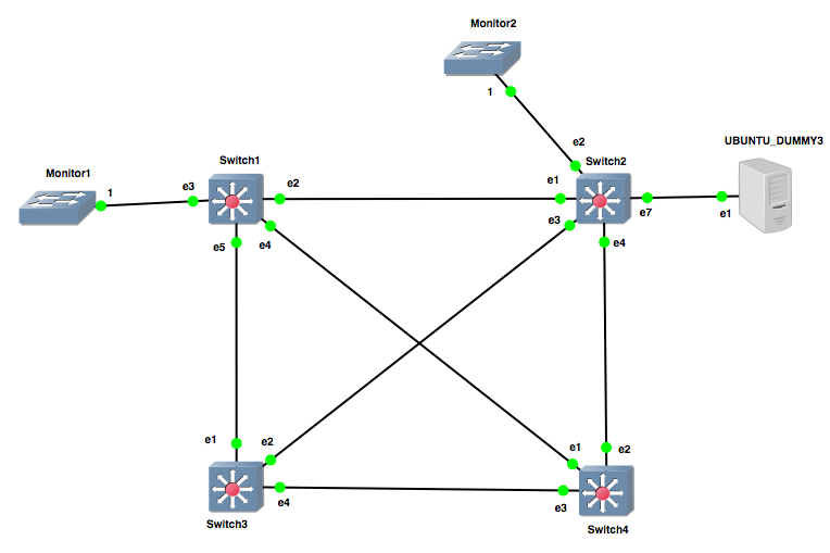
Here is the topology:

EtherSwitches have been added only to capture traffic off monitoring sessions set up on Switch1 and Switch2 to look at in Wireshark.  The Ubuntu server can be ignored for the purposes of this blog entry.

Only VLAN 1 is present on all switches and Switch1 is configured to be the primary root, while Switch2 is configured to be the secondary. Here's the current state of the network:

First it's important to note that only a single thing will trigger a topology change event - the transition of a non-Edge port from a non-Forwarding to a Forwarding state. Why?  Because this newly Forwarding port could possibly provide a better path to a given destination MAC address than there was before, and the CAM table will need to be updated to reflect that and prevent the same MAC being displayed on more than one port.  It sounds strange that a loss of a Forwarding port doesn't trigger a topology change event, but think about it - in a L2 world, you can't have multiple paths to reach a destination. "There can be only one."  Otherwise it would likely mean there is a loop.  Taking that into consideration, if our only path to a destination MAC breaks, we know we can't get there unless another path is created by another port transitioning to Forwarding - which will trigger a topology change event.  Viola - work smarter not harder!

To review the Topology Change process when a switch detects a topology change event:

1. Set tcWhile timer on all non-Edge Designated ports and Root port if it exists
2. Flush MAC addresses learned on ports in step 1
3. Send BPDUs with the Topology Change (TC) flag set on these ports every Hello seconds until tcWhile expires

So let's first look at what happens locally on a switch, as we shut interface Et1 on Switch4 which is its Root Port.  First, I'll ping Switch4 from Switch2, then look at Switch4's CAM table:

Switch4#sh mac address-table 

          Mac Address Table

------------------------------------------------------------------

Vlan    Mac Address       Type        Ports      Moves   Last Move

----    -----------       ----        -----      -----   ---------

   1    0800.274a.33f1    DYNAMIC     Et1        1       0:00:25 ago

Total Mac Addresses for this criterion: 1

We see it learned Switch2's MAC address on Et1. Vice-versa, we look at Switch2's CAM table and see it learned Switch4's MAC on Et1:

Switch2#sh mac address-table

          Mac Address Table

------------------------------------------------------------------

Vlan    Mac Address       Type        Ports      Moves   Last Move

----    -----------       ----        -----      -----   ---------

   1    0800.277b.3066    DYNAMIC     Et1        1       0:00:28 ago

Total Mac Addresses for this criterion: 1

Now, let's do the same process over again, but then shut down Et1 on Switch4. Et1 is Switch4's Root Port, so what should happen is Et2, which is an Alternate Port, should transition to a Forwarding state.  This meets the criteria for a topology change event.

After we shut Et1, we take a look at the spanning tree status on Switch4:

Switch4#sh span

VL1

  Spanning tree enabled protocol rapid-pvst

  Root ID    Priority    4097

             Address     0800.2773.3845

             Cost        4000 (Ext) 0 (Int)

             Port        2 (Ethernet2)

             Hello Time  2.000 sec  Max Age 20 sec  Forward Delay 15 sec

  Bridge ID  Priority    32769  (priority 32768 sys-id-ext 1)

             Address     0800.277b.3066

             Hello Time  2.000 sec  Max Age 20 sec  Forward Delay 15 sec

Interface        Role       State      Cost      Prio.Nbr Type

---------------- ---------- ---------- --------- -------- --------------------

Et2              root       forwarding 2000      128.2    P2p                     

Et3              alternate  discarding 2000      128.3    P2p

Et2 transitioned to a Root role, Forwarding state, which qualifies as a topology change event. Looking at the CAM table of Switch4, we see the previous entry is now gone:

Switch4#sh mac address-table 

          Mac Address Table

------------------------------------------------------------------

Vlan    Mac Address       Type        Ports      Moves   Last Move

----    -----------       ----        -----      -----   ---------

Total Mac Addresses for this criterion: 0

Looking at Switch2, we see the previous entry is also gone as well:

Switch2#sh mac address-table 

          Mac Address Table

------------------------------------------------------------------

Vlan    Mac Address       Type        Ports      Moves   Last Move

----    -----------       ----        -----      -----   ---------

Total Mac Addresses for this criterion: 0

Why did this also happen on Switch2?  If you scroll back up and look at what happens on a switch during a topology change event, you saw that the last item mentioned sending BPDUs with the TC flag set:

Send BPDUs with the Topology Change (TC) flag set on these ports every Hello seconds until tcWhile expires

So once Switch4 detected the topology change, it started firing off BPDUs with the TC flag bit set out its newly-elected Root Port, interface Et2.

Once a switch experiences a local topology change, or learns about one from another switch by receiving a BPDU with the TC flag set on a Root or Designated port, it too will in turn go through the same process.  So let's take a look at what happened on the network holistically:

1. Interface Et1 which was the Root Port for Switch4 is shut down. Switch4 had elected Et2 as an Alternate Port previously, so it immediately transitions the port to the new Root Port. This places Et2 into a Forwarding state which triggers a topology change event, so Switch4 then sets the tcWhile timer and flushes the CAM table entries learned on Et2, and begins sending BPDUs with the TC flag set out the same port. At the same time, Et3 begins receiving superior BPDUs so it is transitions from a Designated Port to an Alternate Port.   
2. Switch2 receives a BPDU with the TC flag set on Et4, so it sets the tcWhile timer, flushes any CAM table entries learned on, and begins sending BPDUs with the TC flag set on its Root and other Designated Port, Et1 and Et3, respectively. Ultimately, the TC BPDU sent from Et3 will be discarded upon reaching Switch3.
3. Switch1 receives a TC BPDU on Et2.  It sets the tcWhile timer, flushes learned CAM table entries, and sends TC BPDUs from its only other remaining active Designated Port, Et5.
4. After interface Et1 on Switch4 was shut down, Switch3 began receiving what it determined to be inferior BPDUs on Et4 due to Switch4 now advertising a higher Root Path Cost (RPC), so Switch3 transitioned the port from an Alternate Port to a Designated Port. Switch3 then receives a TC BPDU on Et1, so it sets the tcWhile timer, flushes any learned CAM table entries, and sends TC BPDUs out its only other Designated Port, Et4 - which will end up being discarded.

At this point, all switches have been informed and made the appropriate changes into a new, loop-free converged topology.  So that's how the topology change process is handled in RSTP!  

BGP in an Arista Data Center

The following is a practical analysis of the use of BGP in the DC on Arista platforms based largely on Petr Lapukhov's work with BGP in hyperscale DCs

Why Layer 3 (L3)?

There are several reasons to run a L3 routing protocol over legacy layer 2 (L2) designs in the data center. Leveraging standards-based routing protocols to avoid vendor lock-in, provide for faster convergence, minimize L2 fault domains, and provide for better traffic engineering.

Extension of L2

Naturally something that comes into question in a L3 switch fabric is, “What if I need L2 adjacency between hosts?” For Arista, the extension of L2 services across a L3 switch fabric is provided by Virtual eXtensible LAN (VXLAN). While closely related, in-depth discussion of the “network overlay” provided by VXLAN is outside the scope.

Why BGP?

Some might question the use of BGP within the data center due to it being designed for, and in the past primarily leveraged as, an EGP. However, BGP provides several benefits in a data center switch fabric, such as:

• Less complexity in protocol design
• Relies on TCP rather than adjacency formation/maintenance and/or flow control
• Less “chatty”
• Supports third-party (recursively-resolved) next-hops
• With proper ASN usage, built-in loop prevention via AS_PATH
• Better support for traffic engineering

General Operations Within the Fabric

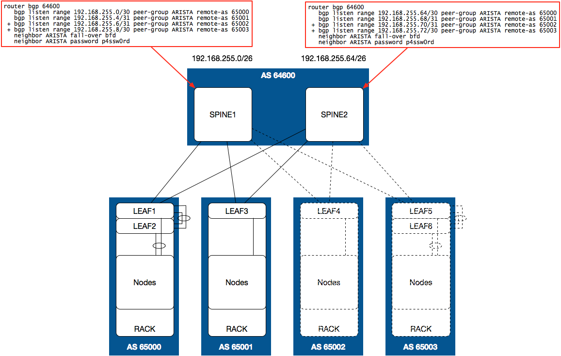
ASN Scheme Option 1(Per-Rack Leaf AS)

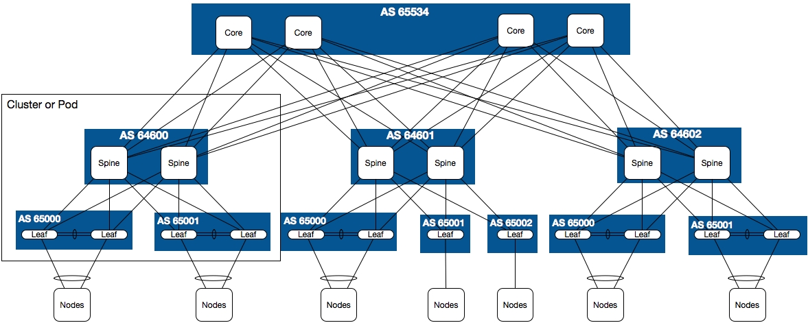
Below is a diagram derived mostly from an IETF Draft that is a joint effort by Facebook, Google, and Arista Networks for very large data centers. It is shown in entirety to help visualize the reuse of ASNs at the leaf layer.

Notice that ASNs are reused at the leaf layer for each “cluster” or “pod”. This is achievable by configuring the leaf switches with allowas-in, and minimizes the need for 4-Byte ASNs which not all vendors support. Loop prevention is provided at the spine layer by placing spine switches within the same AS at each cluster/pod.

Going forward, focus will be on the spine/leaf elements.

ASN Scheme Option 2 (Leaf Layer AS)

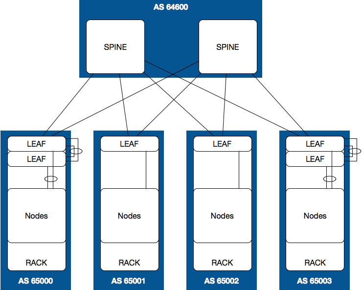
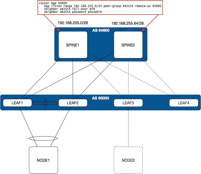
Another option could be to use the same AS at every leaf:

Advantages of this design include less ASN usage, simple configuration templatization, and with that, better support for automation. A disadvantage is losing the ability to trace routes via AS_PATH (At least without additional configuration). These topics are further discussed in later sections.
Intra-AS Spine-to-Spine Reachability

Due to the spine switches being in the same AS, direct reachability from spine-to-spine within the same AS is not supportable without breaking loop prevention within the architecture itself. However, the impact of this is very minimal and should mostly be ignored.

Dynamic Neighbor Discovery

As a data center scales out, it is possible that many more leaf switches will be added. To make life easier, it is very desirable to automate and reduce configuration however possible. BGP dynamic neighbors configured at the spine layer provides a mechanism to dynamically add new leaf switches as BGP peers based on an IP address range. To support this, care must be taken in IP addressing as described in the “IP Addressing and Prefix Advertisement” section.

BGP Dynamic Neighbors with Per-Rack Leaf AS

Below is a diagram depicting the utilization of a separate AS at each rack:

In this configuration, a bgp listen router configuration command is added for each new rack with the IP address range accounting for the routed links going to each leaf switch within the rack. This reduces the amount of required configuration versus static configuration for each individual leaf.

BGP Dynamic Neighbors with Leaf Layer AS

Below, the second option leverages the same AS at every leaf:

In this configuration, a single bgp listen router configuration command is all that is required at each spine. No further configuration is needed at the spine as additional leaf switches are added to the environment. This makes the configuration easy to templatize and automate across all spine switches.

Making it Easy to Automate

It is much easier to automate configuration when it can be applied to a container of devices rather than having to have specific, per-device configuration.

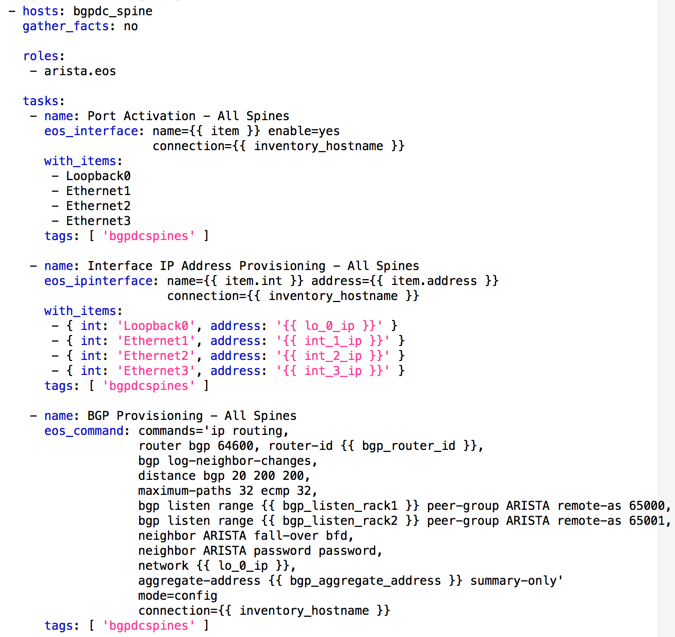
For example, Ansible is a YAML-based automation platform that can be leveraged to push configuration to Arista switches. When configuration is simple and repeatable on as many devices as possible, that configuration can be compartmentalized into a template more easily. Ansible uses “playbooks” which are basically a list of resources and what tasks should be performed on those resources. Below is an excerpt from a playbook showing a single template configuration that could be applied to all spine switches in a per-rack Leaf AS design (Given a whopping two racks, but you get the idea):

In summary, the more configuration you can compartmentalize and template, the less items need to be defined as variables while still being able to be repeated on multiple devices - and still meet requirements of course - the better.

Route Source Tracing via AS_PATH with Leaf Layer AS

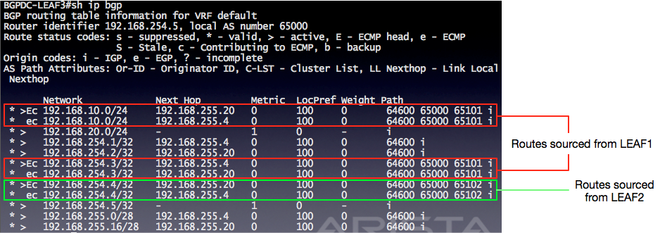
As mentioned earlier, a disadvantage to using the same AS at every leaf is not having the ability to trace routes via AS_PATH:

To get around this, an ASN could be prepended using a route map on each leaf switch, for example:

BGPDC-LEAF1(config)#route-map BGP_PREPEND
BGPDC-LEAF1(config-route-map-BGP_PREPEND)#set as-path prepend 65101

BGPDC-LEAF2(config)#route-map BGP_PREPEND
BGPDC-LEAF2(config-route-map-BGP_PREPEND)#set as-path prepend 65102

Then on both leaf switches, apply the route-map to all advertised routes:

router bgp 65000
neighbor ARISTA route-map BGP_PREPEND out

Now from LEAF3’s perspective, it is easier to see where the routes were sourced from:

IP Addressing and Prefix Advertisement

One challenge that resides in having a layer three (L3) switch fabric in the data center is how to handle your point-to-point routed links between spine and leaf switches. Not advertising them can increase troubleshooting difficulty, but advertising them inefficiently can lead to a large number of /31 entries in the Routing Information Base (RIB) that may become resource-intensive.

As a hypothetical example, if an Arista 7050QX-32 switch were to be used as a spine switch, assuming no ports are used for uplinks to the core or edge, and only 40Gb links are used to connect leaf switches, you would have a total of 32 links with /31 addressing. This means they could be aggregated as follows:

• 16 /30s
• 8 /29s
• 4 /28s
• 2 /27s
• 1 /26

A single /26 can represent all possible point-to-point connections that the particular spine switch could have. So if you started with 192.168.255.0 for your IP addressing on your point-to-point links, you could allocate contiguous blocks of IP addresses starting with 192.168.255.0/26 for the first spine switch, 192.168.255.64/26 for the second spine switch, and so on. Then on each spine switch, only advertise its loopback and the aggregate with the aggregate-address summary-only BGP router configuration command.

What this will ultimately look like from the leaf layer perspective is an optimized RIB containing the loopbacks of all switches in the fabric, and a single additional entry per spine switch to reach point-to-point IP addresses for troubleshooting purposes.

To help visualize, consider a scenario where two spine switches are connected to just three leaf switches. The two spine switches have been configured to advertise every leaf connection, like so:

BGPDC-SPINE1(config-router-bgp)#sh active
router bgp 64600
router-id 192.168.254.1
bgp log-neighbor-changes
distance bgp 20 200 200
maximum-paths 32 ecmp 32
bgp listen range 192.168.255.0/24 peer-group ARISTA remote-as 65000
neighbor ARISTA peer-group
neighbor ARISTA fall-over bfd
neighbor ARISTA password 7 6x5GIQqJNWigZDc2QCgeMg==
neighbor ARISTA maximum-routes 12000
network 192.168.254.1/32
network 192.168.255.0/31
network 192.168.255.2/31
network 192.168.255.4/31

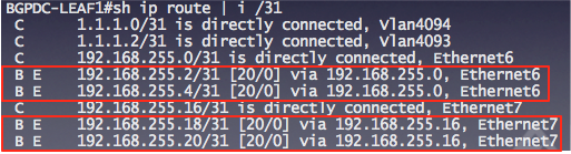
Looking at the routing table of LEAF1, there are a number of /31 entries learned via BGP:

As you can imagine, in larger environments, the number of entries could be excessive. Instead, the spine switches can configured with the aggregate-address router configuration command:

BGPDC-SPINE1(config-router-bgp)#sh active
router bgp 64600
router-id 192.168.254.1
bgp log-neighbor-changes
distance bgp 20 200 200
maximum-paths 32 ecmp 32
bgp listen range 192.168.255.0/24 peer-group ARISTA remote-as 65000
neighbor ARISTA peer-group
neighbor ARISTA fall-over bfd
neighbor ARISTA password 7 6x5GIQqJNWigZDc2QCgeMg==
neighbor ARISTA maximum-routes 12000
network 192.168.254.1/32
aggregate-address 192.168.255.0/28 summary-only


The same output from LEAF1 now shows no /31 entries learned from BGP:

Instead, there is a single /28 entry from each spine learned via BGP:

BGP at the Spine Layer

The Need for Fast Failure Detection

In a BGP switch fabric it is critical for failures to be detected as quickly as possible at the spine layer. Consider the following hypothetical scenario:

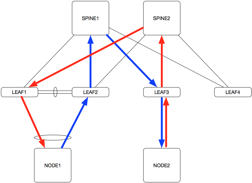
NODE1 is communicating with NODE2. LEAF1 and LEAF2 are MLAG peers. In an ECMP-routed switch fabric, asymmetric routing can occur, where NODE1’s traffic flow is taking the path through LEAF2, while the return traffic is taking the path through LEAF1. This is fine for now, but let’s consider what happens when LEAF1 is rebooted:

With default behavior of MLAG, when LEAF1 finishes rebooting and re-establishes the MLAG session with LEAF2, LEAF1 will place all non-peer-link interfaces into the err-disable state for 300 seconds (five minutes) in order to allow the topology to reconverge. So including the reboot, you’re looking at ~7 minutes or so before the switch begins forwarding again. Even though you have a redundant gateway provided by LEAF2, the reboot of LEAF1 would actually create a problem when combined with the fact that the spine switches are using default configuration in this particular situation of asymmetric routing. Default BGP keepalive and hold timers are 30 seconds and 180 seconds, respectively, so for 180 seconds (3 minutes), the spine switches will still consider LEAF1 an established BGP neighbor, and still consider the path to LEAF1 a viable route even though it’s clearly not. So for any flow that gets hashed to this path, the traffic is effectively blackholed. BGP timers could be modified to provide some relief, but failover time may still be considered unacceptable, in addition to the possibility of introducing instability of the network to BGP peer flapping.

By default, Arista switches will immediately tear down an eBGP neighbor adjacency when the interconnecting link goes down. This alleviates the issue described above. To further improve failure detection, Bidirectional Forwarding Detection (BFD) should also be leveraged. BFD is a very simple, low overhead Hello protocol that works in conjunction with BGP to provide sub-second failure detection. BFD adds additional protection in “gray” failure conditions such as would possibly be seen with a degraded fiber strand. The interface status may remain up and therefore not trigger the eBGP neighborship tear-down, but not pass traffic intermittently or at all - which in those cases network performance can suffer while the BGP keepalive/hold-down mechanism by itself may or may not be of much help.

BGP at the Leaf Layer

MLAG - To Peer or not to Peer

When running a pair of leaf switches in an MLAG configuration with VARP, you want to peer the two leaf switches. Although unlikely to actually happen, consider the following failure scenario:

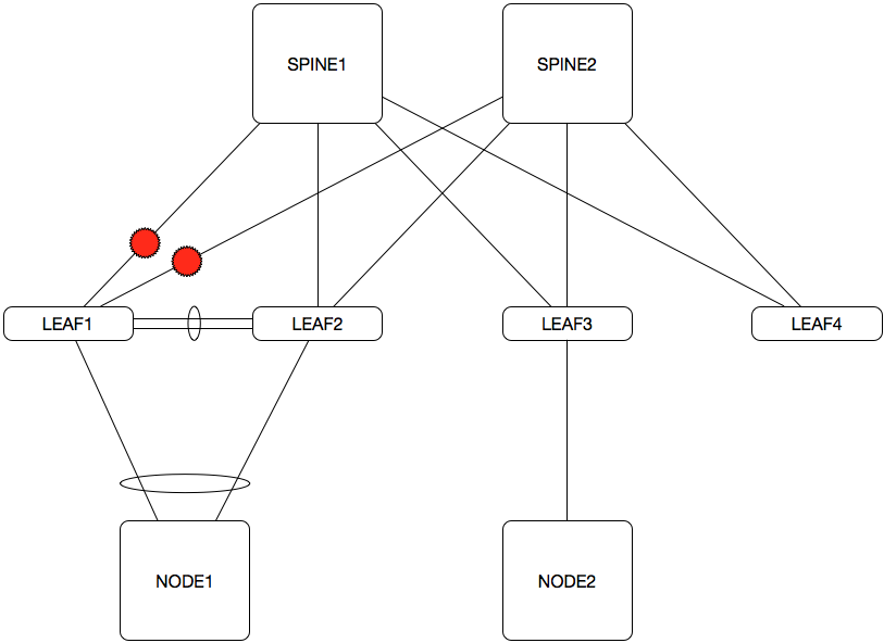
NODE1 is communicating with NODE2. LEAF1 and LEAF2 are MLAG peers and are configured to run VARP to provide an active/active redundant first hop gateway for NODE1, but they are not BGP peers. On LEAF1, both of its uplinks have failed. While both SPINE1 and SPINE2 would certainly notice this failure and reconverge, some things will not be affected, such as:

• MLAG running between LEAF1 and LEAF2 would not notice any change, and continue functioning as normal, which in turn means that the port-channel between NODE1 and LEAF1/LEAF2 would remain up and function as normal
• VARP would continue to function as normal

This is important because traffic leaving NODE1 that gets hashed to LEAF2 would be fine, but any traffic hashed to LEAF1 would effectively be blackholed:

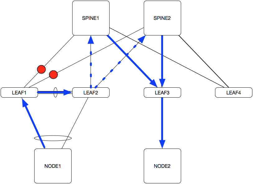
Peering LEAF1 and LEAF2 alleviates this. Traffic hashed to LEAF1 would follow the only remaining route pointing to LEAF2, and then be ECMP-routed to the spine layer:

Additionally, when this failure scenario doesn’t exist, you don’t have to worry about having a suboptimal path because without the failure described above, the path through the peering leaf switch is longer than those directly connected to the spine layer:

Optimizations

update wait-for-convergence

The update wait-for-convergence BGP router configuration command basically prevents BGP from programming routes into hardware and from advertising routes until a convergence event is resolved. A convergence event can occur when initializing BGP for the first time, clearing the BGP process, terminating the Rib agent, etc. The benefit this provides is reduced CPU churn from repeatedly programming routes into and out of hardware during a convergence event.

Best practice is to only use this on spine switches. Enabling this on leaf switches (especially leaf switches acting as host gateways) can result in traffic being blackholed until BGP finishes installing routes in hardware.

NOTE: Enabling this feature in vEOS will cause routes not to be advertised.

update wait-install

The update wait-install BGP router configuration command prevents routes from being advertised to peers until they are programmed in hardware, and that hardware sends an “Ack” to software. This prevents traffic being dropped in situations where routes are advertised, but they aren’t programmed yet in hardware.

NOTE: Enabling this feature in vEOS will cause routes not to be advertised.

ip hardware fib next-hop update event bfd

The ip hardware fib next-hop update event bfd global configuration command allows BFD to remove an interface that went down from next-hop entries of routes using it in hardware. The benefit is reduced traffic loss compared to the normal operation of BFD which is to bring down the BGP neighborship and recompute the next-hop for all routes using the interface which went down and then reprogram hardware. This is a default configuration whenever BFD is enabled.

ip hardware fib route unprogrammed parent-drop

The ip hardware fib route unprogrammed parent-drop global configuration command makes it so that if a more specific route cannot be programmed in hardware for whatever reason, its parent route will be programmed to point to a drop index (similar to null0). This is default behavior.

NOTE: This is not really an optimization, and is instead more of a feature. It should be noted that this will result in traffic being black-holed rather than being forwarded on to possibly undesirable destinations which is the “benefit” of this feature. An unfortunate side effect is that if there is no other parent route, the default route will be pointed to a drop index instead. In summary, if there isn’t a need to prevent traffic being routed using parent routes when a more specific route cannot be programmed, it is recommended to disable this feature with the “no” form of the same command.

Sources

• RFC 4271, “A Border Gateway Protocol 4 (BGP-4)”, https://tools.ietf.org/html/rfc4271
• “Use of BGP for routing in large-scale data centers”, http://datatracker.ietf.org/doc/draft-ietf-rtgwg-bgp-routing-large-dc/
• “Understanding BGP Convergence”, http://blog.ine.com/2010/11/22/understanding-bgp-convergence/

Configuration Excerpt Examples

Configuration examples are from a small-scale switch fabric created using virtual Extensible Operating System (vEOS) version 4.15.0F.

Per-Rack Leaf AS (Option 1)

SPINE1

interface Ethernet1
no switchport
ip address 192.168.255.0/31
!
interface Ethernet2
no switchport
ip address 192.168.255.2/31
!
interface Ethernet3
no switchport
ip address 192.168.255.4/31
!
interface Loopback0
ip address 192.168.254.1/32
!
ip routing
no ip hardware fib route unprogrammed parent-drop
!
router bgp 64600
router-id 192.168.254.1
update wait-for-convergence
update wait-install
bgp log-neighbor-changes
distance bgp 20 200 200
maximum-paths 32 ecmp 32
bgp listen range 192.168.255.0/30 peer-group ARISTA remote-as 65000
bgp listen range 192.168.255.4/31 peer-group ARISTA remote-as 65001
neighbor ARISTA peer-group
neighbor ARISTA fall-over bfd
neighbor ARISTA password p4ssw0rd
network 192.168.254.1/32
aggregate-address 192.168.255.0/28 summary-only

LEAF1

vlan 10
name HOST_10
!
vlan 4093
name BGP_PEER
trunk group BGP_PEER
!
vlan 4094
name MLAG
trunk group MLAG
!
interface Port-Channel1
switchport mode trunk
switchport trunk group BGP_PEER
switchport trunk group MLAG
!
interface Ethernet5
channel-group 1 mode active
!
interface Ethernet6
no switchport
ip address 192.168.255.1/31
!
interface Ethernet7
no switchport
ip address 192.168.255.17/31
!
interface Loopback0
ip address 192.168.254.3/32
!
interface Vlan10
ip address 192.168.10.2/24
ip virtual-router address 192.168.10.1/24
!
interface Vlan4093
ip address 1.1.1.2/31
!
interface Vlan4094
ip address 1.1.1.0/31
!
ip routing
no ip hardware fib route unprogrammed parent-drop
!
!
route-map BGP_PREPEND permit 10
set as-path prepend 65101
!
router bgp 65000
router-id 192.168.254.3
update wait-install
bgp log-neighbor-changes
distance bgp 20 200 200
maximum-paths 32 ecmp 32
neighbor ARISTA peer-group
neighbor ARISTA remote-as 64600
neighbor ARISTA allowas-in 1
neighbor ARISTA fall-over bfd
neighbor ARISTA route-map BGP_PREPEND out
neighbor ARISTA password p4ssw0rd
neighbor 1.1.1.3 peer-group ARISTA
neighbor 1.1.1.3 remote-as 65000
neighbor 1.1.1.3 next-hop-self
neighbor 192.168.255.0 peer-group ARISTA
neighbor 192.168.255.16 peer-group ARISTA
network 192.168.10.0/24
network 192.168.254.3/32

Leaf Layer AS (Option 2)

SPINE1

interface Ethernet1
no switchport
ip address 192.168.255.0/31
!
interface Ethernet2
no switchport
ip address 192.168.255.2/31
!
interface Ethernet3
no switchport
ip address 192.168.255.4/31
!
interface Loopback0
ip address 192.168.254.1/32
!
ip routing
no ip hardware fib route unprogrammed parent-drop
!
router bgp 64600
router-id 192.168.254.1
update wait-for-convergence
update wait-install
bgp log-neighbor-changes
distance bgp 20 200 200
maximum-paths 32 ecmp 32
bgp listen range 192.168.255.0/24 peer-group ARISTA remote-as 65000
neighbor ARISTA peer-group
neighbor ARISTA fall-over bfd
neighbor ARISTA password p4ssw0rd
neighbor ARISTA maximum-routes 12000
network 192.168.254.1/32
aggregate-address 192.168.255.0/28 summary-only

LEAF1

vlan 10
name HOST_10
!
vlan 4093
name BGP_PEER
trunk group BGP_PEER
!
interface Port-Channel1
switchport mode trunk
switchport trunk group BGP_PEER
switchport trunk group MLAG
!
interface Ethernet5
channel-group 1 mode active
!
interface Ethernet6
no switchport
ip address 192.168.255.1/31
!
interface Ethernet7
no switchport
ip address 192.168.255.17/31
!
interface Loopback0
ip address 192.168.254.3/32
!
interface Vlan10
ip address 192.168.10.2/24
ip virtual-router address 192.168.10.1
!
interface Vlan4093
ip address 1.1.1.2/31
!
ip routing
no ip hardware fib route unprogrammed parent-drop
!
route-map BGP_PREPEND permit 10
set as-path prepend 65101
!
router bgp 65000
router-id 192.168.254.3
update wait-install
bgp log-neighbor-changes
distance bgp 20 200 200
maximum-paths 32 ecmp 32
neighbor ARISTA peer-group
neighbor ARISTA remote-as 64600
neighbor ARISTA allowas-in 1
neighbor ARISTA fall-over bfd
neighbor ARISTA route-map BGP_PREPEND out
neighbor ARISTA password p4ssw0rd
neighbor 1.1.1.3 peer-group ARISTA
neighbor 1.1.1.3 remote-as 65000
neighbor 1.1.1.3 next-hop-self
neighbor 192.168.255.0 peer-group ARISTA
neighbor 192.168.255.16 peer-group ARISTA
network 192.168.10.0/24
network 192.168.254.3/32

SPAN Destination ports and VLAN Membership

Recently at work, a discussion sprouted up around how to handle/configure local session Switched Port Analyzer (SPAN) destination ports.  A suggestion was made to create a new VLAN just for these SPAN destination ports and place them there.  The justification was that they would be out of VLAN 1, and easily identifiable.  Personally I thought it was a waste of a VLAN for a few simple SPAN destination ports, as SPAN destination ports do not participate in spanning tree, and do not forward traffic.  However, ultimately in this case it was a good decision due to security requirements.
Some key characteristics to know about SPAN destination ports:

• A destination port can be a physical port that is assigned to an EtherChannel group, even if the EtherChannel group has been specified as a SPAN source. The port is removed from the group while it is configured as a SPAN destination port.
  
• The port does not transmit any traffic except that traffic required for the SPAN session unless learning is enabled.
  
• The state of the destination port is up/down by design. The interface shows the port in this state in order to make it evident that the port is currently not usable as a production port.
  
• If ingress traffic forwarding is enabled for a network security device. The destination port forwards traffic at Layer 2.
  
• A destination port does not participate in spanning tree while the SPAN session is active.
  
• When it is a destination port, it does not participate in any of the Layer 2 protocols (STP, VTP, CDP, DTP, PagP).
  
• A destination port that belongs to a source VLAN of any SPAN session is excluded from the source list and is not monitored.
  
• A destination port receives copies of sent and received traffic for all monitored source ports. If a destination port is oversubscribed, it can become congested. This congestion can affect traffic forwarding on one or more of the source ports.
  
• When you configure a port as a SPAN destination, it is dedicated for use only by the SPAN feature.
  
• Destinations, by default, cannot receive any traffic. With Release 12.2(33)SXH and later releases, you can configure Layer 2 destinations to receive traffic from any attached devices.
  
• Destinations, by default, do not transmit anything except SPAN traffic. Layer 2 destinations that you have configured to receive traffic can be configured to learn the Layer 2 address of any devices attached to the destination and transmit traffic that is addressed to the devices.

Sources:
http://www.cisco.com/en/US/products/hw/switches/ps708/products_tech_note09186a008015c612.shtml#charac_dest
http://www.cisco.com/en/US/docs/switches/lan/catalyst6500/ios/12.2SX/configuration/guide/span.html#wp1020380
Some of the points above seem like repeats and that was done on purpose to emphasize the point.  Probably the most important point is the one about the port being in an Up/Down status.  To me, this would naturally indicate that it is doing nothing outside of its SPAN function.

Spanning Tree Exercise and Revisiting Root Guard

This was actually spurned from a comment I received on another one of my blog posts that you can find here.  Seeing that comment, I white boarded it and realized that I may have been completely wrong in regards to how Root Guard could “break a network”. 

Let’s say we have the following topology:

• Core 1 is the root for VLAN 10 with a configured priority of 4096, and is the secondary root for VLAN 20 with a configured priority of 8192.  We alternate this with Core 2 in order to load balance VLAN traffic.
• Access 3 and 4 are left in default configuration regarding spanning tree.
• Two workstations are present – one in VLAN 10, and another in VLAN 20.  Their default gateways are SVIs that are on the Core switches.
• For simplicity, switch MAC addresses are the number contained in their names.  Example: Access 4’s MAC address is “4”.
• All link costs are the same.
• All links between switches are trunks transporting all VLANs.

Let’s work through the spanning tree topologies.

Core 1 – Root bridge for VLAN 10.  All ports designated.

Core 2 – Port 1 will be a root port due to lowest cost to root. Since the cost to reach root for Core 2, Access 3, and Access 4 are equal, and a root port exists, ports 2 and 3 will be designated due to Core 2 having the lowest bridge ID (STP tie-breaker).  We know this by calculating the bridge IDs:

• Core 2  - MAC Address (2) + VLAN ID (10) + Priority (8192) = 8204
• Access 3 – MAC Address (3) + VLAN ID (10) + Priority (32768) = 32781
• Access 4 – You get the idea.

Access 3 and 4 – Port 1 will be the root port leaving port 2 as blocking since there are already designated ports on those links belonging to Core 2.

VLAN 10	Port 1	Port 2	Port 3
Core 1	Designated	Designated	Designated
Core 2	Root	Designated	Designated
Access 3	Root	Blocking	N/A
Access 4	Root	Blocking	N/A

And for VLAN 20:

VLAN 20	Port 1	Port 2	Port 3
Core 1	Root	Designated	Designated
Core 2	Designated	Designated	Designated
Access 3	Blocking	Root	N/A
Access 4	Blocking	Root	N/A

Now we can see how traffic will flow from each workstation to each other.

VLAN 10 Workstation to VLAN 20 Workstation:

1. Traffic leaves VLAN 10 Workstation and hits VLAN 10 SVI on Core 1
2. Multilayer switched to VLAN 20 within Core 1.
3. Hit Core 2 since the link directly to Access 4 is blocked on VLAN 20.
4. Traverse Access 4 to reach VLAN 20 Workstation.

And now we move to the million dollar question from my previous blog article.  Let’s say we have Root Guard configured on ports 2 and 3 on both Core 1 and Core 2.  What happens when we lose the link between the Core switches? First it may warrant to discuss what happens without Root Guard in place:

Core 1 – Root bridge for VLAN 10 – all remaining ports remain designated.

Core 2 – Since the cost to root is the same going through either Access 3 or Access 4, port 2 will transition to a root port due to, again, Access 3 having the lowest bridge ID. Port 3 will transition to a blocking state since Access 4 now has the lowest cost to reach root for that link.

Access 3 – Port 1 remains a root port.  Port 2 transitions to a designated port since Access 3 has the lowest cost to reach root on that link.

Access 4 – Port 1 remains a root port.  Port 2 transitions to a designated port since Access 4 has the lowest cost to reach root on that link.

VLAN 10	Port 1	Port 2	Port 3
Core 1	Down	Designated	Designated
Core 2	Down	Root	Blocking
Access 3	Root	Designated	N/A
Access 4	Root	Designated	N/A

And for VLAN 20:

VLAN 20	Port 1	Port 2	Port 3
Core 1	Down	Root	Blocking
Core 2	Down	Designated	Designated
Access 3	Designated	Root	N/A
Access 4	Designated	Root	N/A

This has some pretty drastic results:

The path for the blue Workstation to the red Workstation is pretty straight-forward.  But check out the path from the red Workstation to the blue one:

1. Traffic from the VLAN 10 Workstation hits the VLAN 10 SVI on Core 1 as usual.
2. Multilayer switched to VLAN 20 within Core 1, again, as usual.
3. Here’s where it gets interesting.  The link between Core 1 and Core 2 is physically down, and STP is blocking on port 3 for VLAN 20, so this traffic must go back down to Access 3.
4. Traffic traverses Core 2 and Access 4 before finally reaching its destination.

Now let’s see what happens when we enable Root Guard on Core 1 and Core 2’s ports 2 and 3:

• Core 1 begins receiving superior BPDUs on VLAN 20 on ports 2 and 3, so it places those ports in root-inconsistent.
• Core 2 begins receiving superior BPDUs on VLAN 10 on ports 2 and 3, so it places those ports in root-inconsistent.

VLAN 10	Port 1	Port 2	Port 3
Core 1	Down	Designated	Designated
Core 2	Down	Root-Inconsistent	Root-Inconsistent
Access 3	Root	Designated	N/A
Access 4	Root	Designated	N/A

 

VLAN 20	Port 1	Port 2	Port 3
Core 1	Down	Root-Inconsistent	Root-Inconsistent
Core 2	Down	Designated	Designated
Access 3	Designated	Root	N/A
Access 4	Designated	Root	N/A

Now lets take a look at traffic flow from the red Workstation to the blue:

1. Traffic leaves the VLAN 10 Workstation and hits the VLAN 10 SVI on Core 1
2. Multilayer switched to VLAN 20 within Core 1
3. Uh oh – port 1 is physically down and ports 2 and 3 are down for VLAN 20 thanks to Root Guard.  The traffic has no where to go!

Welp – guess I wasn’t wrong after all.  This appears to be a corner case scenario because if it were only a single instance of spanning tree there would be no issue.  Even in this scenario, intra-VLAN communication would be fine, but this does break inter-VLAN communication.

OSPF Adjacency Building Process

Ever curious regarding how two routers configured for OSPF become fully adjacent?  The following diagram of the process was modeled directly from RFC 2328, and the steps described gleaned from the Routing TCP/IP Vol I book.  Since we can see mention of a DR, this example must be based on a multi-access network.

1. RT1 becomes active and sends a Hello.  At this point, RT1 hasn’t seen any neighbors, so it reports such and sets its DR and BDR fields to 0.0.0.0.
2. Upon receipt by RT2, RT2 will build a data structure for RT1 and set RT1’s state to Init.  RT2 will then send a Hello packet reporting that it has seen RT1, and will report itself as the DR.
3. RT1 now sees its own RID in the received Hello packet from RT2, so RT1 will now create a data structure for RT2 and set its state to ExStart.  RT1 then begins Master/Slave negotiation with a DD packet with a sequence number of “x”, the Init bit set  to indicate that it is the start of an exchange, the More bit set to indicate that it is not the last DD packet to be sent, and lastly with the MS-bit set to indicate that RT1 wants to be the Master.  No LSA summaries are provided just yet – this is purely for Master/Slave negotiation.
4. Upon receipt of RT1’s DD packet, RT2 sets RT1’s state to ExStart.  RT2 then sends a DD with a sequence number of “y”, and the MS-bit set since RT2 has a higher RID in this example.
5. RT1 agrees that RT2 is the Master and sets its state to Exchange. RT1 informs RT2 of its agreement by sending a DD packet with a sequence number “y” that matches what was sent from RT2 in step 4.  The MS-bit will now be set to 0, and here is where we’ll start to see LSA summaries provided by RT1.
6. RT2 now sets RT1’s state to Exchange as well and sends a DD packet containing LSA headers from its Link State Summary list and increments the DD sequence number to “y+1”.
7. RT1 acknowledges this by sending an acknowledgement with the same sequence number that it received in the DD packet from RT2.  It also begins taking the LSA summaries it received and building a Link State Request list.  This process repeats until RT2 sends the last of its LSA summaries and sets the More bit to 0.
8. Once RT1 receives the last of RT2s LSA summaries and acknowledges it knowing that it has sent the last of its own LSA summaries, the Exchange state process is complete.  Now RT1 will begin processing the LSA summaries it has added to its Link State Request list and transition to the Loading state.
9. Once RT2 receives RT1’s last DD packet, RT2 then sets RT1s’s state to Full because RT2 has no entries in its own Link State Request list.
10. RT1 will send Link State Requests for all entries in its Link State Request list and RT2 will send Link Sate Update packets until RT1’s list is empty.  At that point, it sets RT2 to Full, and the adjacency is complete.

OSPF Link State Advertisements (LSAs) and Areas – Part II

For a table describing the different LSA types, check out the first post of this series.

In the first part of the series, we looked at LSA Types 1, 2, and 3 – Router, Network, and Network Summary, respectively.  To move on to the next two LSA types, we need to bring in another Autonomous System (AS).  In the diagram below, we’ve added R5 which has an interface in EIGRP AS 1, and is redistributing that into OSPF Area 4.  The fact that R5 has an interface inside of the OSPF AS, as well as the EIGRP AS, makes R5 an Autonomous System Boundary Router (ASBR). 

The EIGRP-oriented subnet that is being redistributed is considered an external route to the OSPF domain, so a Type 5 LSA, or ASBR External, is flooded into OSPF Area 4 containing a LSID and netmask of the subnet, plus the External Type. This important because it tells other routers whether or not to add the internal link costs within the OSPF domain to the metric to reach that subnet.  A type 2 external route specifies that only the external cost is taken into consideration.

When R2 catches wind of this, it will generate a Type 4 LSA, or ASBR Summary, and flood it into Area 0 as well as the Type 5 LSA.  The contents of the Type 4 LSA are mostly just the LSID of the ASBR’s RID and the metric reach it.

For  other routers to reach this External Type 2 route, they just take metric provided in the Type 5 LSA (20) – no questions asked.

However if it were an External Type 1 route, each router must determine its cost to reach it taking into account the link costs along the way.

So in this example, if R1 needed to reach 172.16.5.0/24 as an External Type 1 route, it would first add the cost to reach R2 (The ABR) [Similar to what it would do to determine cost to an intra-area (IA) route utilizing a Type 3 LSA] to the cost to reach the ASBR as listed in the Type 4 LSA.  Finally, it would then add the cost listed in the Type 5 LSA for that subnet.

Cost to reach ABR (1) + Cost to reach ASBR (2) + Cost in Type 5 LSA (20) = 23

Stubby.. Totally Stubby… Not-So-Stubby… Totally Not-So-Stubby….

While there are several iterations of a stubby area, with varying mechanics behind them, they all serve mostly a single purpose – to reduce overhead.

  

Once R6 is added and area 6 is configured as a stubby area, two major things happen:

• R3 (An ABR for area 6) will still receive, but stop flooding Type 5 LSAs into area 6.  Notice that R6’s routing table does not include R5’s EIGRP-oriented subnet (172.16.5.0/24)
• R3 injects a default route into area 6

So we can see here that the logic is, hey, there’s only going to be one way to get out of this area, so let’s reduce the size of the LSDB and make things easier by just injecting a default route into the area and calling it a day.  Imagine if R5 had 100 subnets hanging off of it in the EIGRP AS – if R6 wasn’t in a stubby area, those 100 routes would be added to its LSDB and in the routing table.  Why do that if we can just inject a default route and not advertise these external routes into the area – effectively accomplishing the same thing?  If R6 needs to hit any of these external routes, it just uses the default route to the ABR who knows how to get there, and greatly reduce the size of R6’s LSDB and routing table all at the same time!

A “totally” stubby area takes this concept even further by also not flooding Type 3 LSAs.  What’s kind of interesting about that statement though is that the default route R3 injects into the stubby area is a Type 3 LSA.

A Not-So-Stubby Area (NSSA) simply allows you to redistribute external routes if needed.  A special type of LSA is used in this situation – a Type 7, or NSSA External.

This will be generated by the now ASBR, R6, who is redistributing its connected 192.168.6.0/24 subnet.  As depicted above, once it reaches the ABR, R3, it will convert this LSA into a Type 5 before flooding it into area 0, so you will only see Type 7 LSAs in a NSSA.